Neural Triangular Transport

A project for MIT course 6.7960

Original work by Daniel Sharp

All code is available at this repository.

U-substitution and Monte Carlo

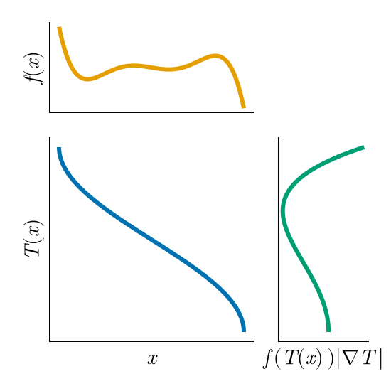
Transforming variables for integration is as old as calculus itself, and is commonly introduced to students as $u$-substitution. While old and elementary, it is obviously still useful across many fields; I address its application to generative modeling here. Given a function $f:\mathbb{R}^d\to\mathbb{R}$, we can express the antiderivative of it using some change of variables $T:\mathbb{R}^d\to\mathbb{R}^d$ as $$\int_\Omega f(x)\ dx = \int_{T^{-1}(\Omega)} f(T(z)) |\nabla T|\ dz,$$ where $T^{-1}(\Omega)$ is the preimage of the domain under $T$; this is visualized below.

We extend this to a target distribution of interest $\pi$ which we might only have data from. Generally, a change of variables under some invertible map $S:\mathbb{R}^d\to\mathbb{R}^d$ is beneficial when given simple reference pdf $\eta$ that we understand well (e.g., uniform or Gaussian) and have

$$\begin{aligned} \int f(x)\ d\pi(x) &= \int f(x)\ dS^\sharp\eta(x)\\ &= \int f(x)\ \eta(S(x))\,|\nabla S(x)|, dx\\ &= \int f(S^{-1}(z))\ d\eta(z) \end{aligned}$$

where $S^\sharp\eta = \eta\circ S |\nabla S|$ is the pullback of $\eta$ under map $S$ (and $|\nabla S|$ is the determinant of the Jacobian of $S$). If we want to estimate expectation $\mathbb{E}_\pi[f]$, we can sample $Z^{(i)}\sim\eta$ i.i.d., deterministically calculate $X^{(i)}\sim S^{-1}(Z^{(i)})$, and perform a Monte Carlo estimate

\[\mathbb{E}_{\pi}[f] \approx \frac{1}{N} \sum_{i=1}^{N} f(X^{(i)}) =\frac{1}{N}\sum_{i=1}^N f(S^{-1}(Z^{(i)})).\]

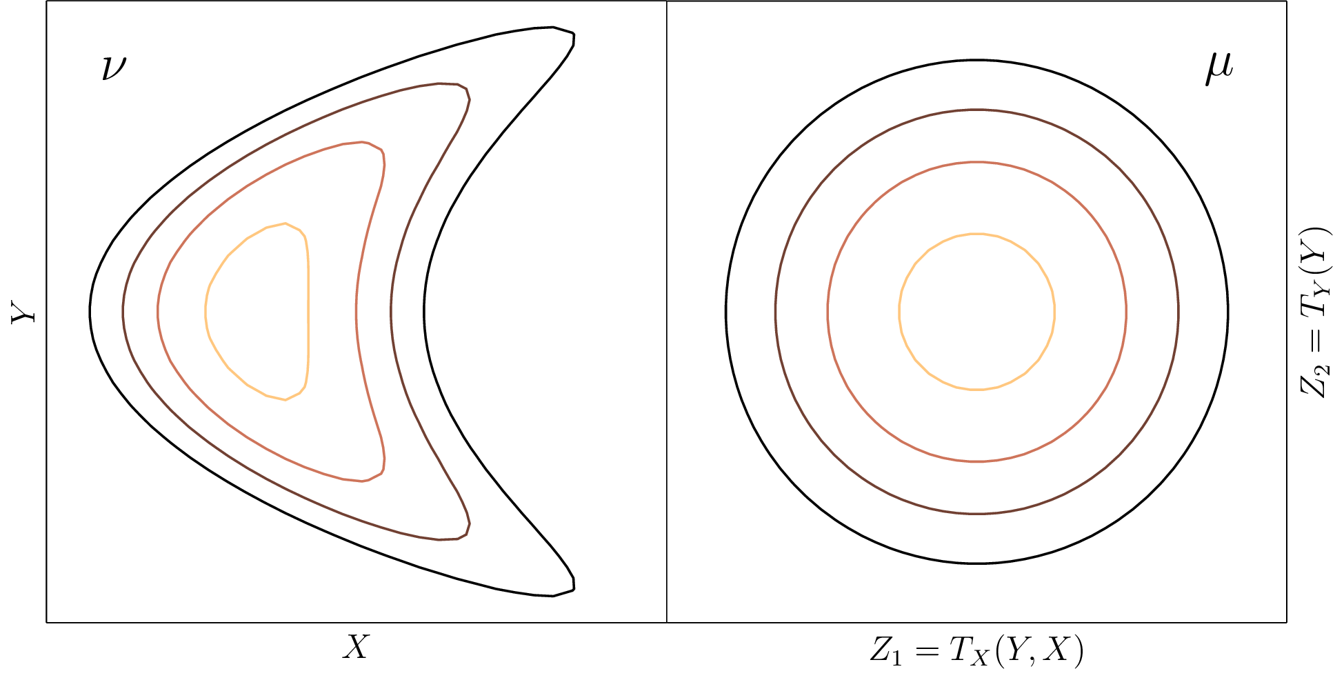
Below is a two-dimensional coupling of pdfs $\mu,\nu$.

Connections to generative modeling

The expressions above provide connections to common deep learning methods. In particular,

• In traditional autoencoders, $S$ is the encoder, $S^{-1}$ is the decoder, and $\eta$ will be the data distribution of the latent space. Obviously, it is not easy to know $\eta$.
• In variational autoencoders (VAEs), we keep $S$ as encoder, $S^{-1}$ as decoder, and $\eta$ is some well-known reference, often understood as Gaussian!
• Diffusion models do not have deterministic $S$ and $S^{-1}$, but we intuit $S$ as the forward diffusion and $S^{-1}$ is the reverse diffusion.
• Similarly, many flow-based methods will act similar to diffusion models in one way or another, though may be induced by deterministic dynamics.
• More "traditional" methods here would be the genre of optimal transport (OT) and the like, often creating mappings $S$ between two different target distributions (i.e., $\eta$ may not be simple). Sinkhorn's algorithm gives a method for estimating a regularized version of $S$ and $S^{-1}$.

All these use different strategies to circumvent the difficulty of creating multidimensional mappings that are invertible. For this reason, I consider methods that learn the map $S$ and provide an architecture to then derive $S^{-1}$. Often, these fall into bins such as invertible neural networks, (continuous) normalizing flows, with related methods such as montone generative adversarial networks, input-convex neural networks, neural-spline flows, etc.

How to sample in one dimension

If your eyes glazed over reading the soup of indeipherable names above, you hopefully have taken away that there is no single $S$ that we can find! Many fall into one of two categories: the authors believe it has a mathematical relevance or the mechanism ensures computational tractability. We pursue the latter case of computational convenience by extending a simple method for one-dimensional sampling.

Consider uniform reference $\eta = U(0,1)$, so $S$ takes a scalar drawn from target $\pi$ and outputs a scalar distributed uniformly on $(0,1)$. We define the cumulative distribution function (CDF) of $\pi$ as $ F_\pi(x) = \int_0^t\pi(t)\ dt$. Therefore, $$\begin{aligned}\int f(x)\ d\pi(x) &= \int f(x)\ F^\prime_\pi(x)\ dx\\ &= \int f(F_\pi^{-1}(z))\ F_\pi^\prime(F_\pi^{-1}(z))\ dF_\pi^{-1}(z)dz\\ &= \int f(F_\pi^{-1}(z)) \ d\eta(z) \end{aligned},$$ given by the inverse function theorem, where we know that $F_{\pi}$ is monotone and thus invertible. For $\mathrm{supp}\pi=(0,1)$, we use $S(x) = F_\pi(x) = \int_0^x \pi(t)\ dt$.

How to sample in multiple dimensions

We can factorize arbitrary pdf $\pi:\mathbb{R}^d\to\mathbb{R}^+$ into conditionals via $$\pi(x) = \pi^{(1)}(x_1)\pi^{(2)}(x_2|x_1)\pi^{(3)}(x_3|x_{1:3})\cdots\pi^{(d)}(x_d|x_{1:d}),$$ with numpy-like notation $x_{i:j} = (x_i,\ldots,x_{j-1})$. For fixed index $j$ and given $x_{1:j}$ (i.e., fixed first $j-1$ variables), we sample $x_j$ by inverting the conditional CDF $$F_{\pi^{(j)}}(x_j;x_{1:j}) = \int_0^{x_j} \pi^{(j)}(t|x_{1:j})\ dt.$$ Of course, $F_{\pi^{(j)}}$ is parameterized by $x_{1:j}$ and this form is slightly simplified by $\eta = U(0,1)^j$, but it serves as motivation for how we parameterize our model.

For given reference pdf $\eta$ as a product measure, i.e., $\eta(x) = \prod_{j=0}^{d} \eta^{(j)}(x_j)$, a triangular transport map $S:\mathbb{R}^d\to\mathbb{R}^d$ is an invertible function with $j$th output $[S(x)]_j = S_j(x_j;x_{1:j})$ satisfying $S_{j}(\cdot; x_{1:j})^\sharp \eta_j = \pi^{(j)}(\cdot|x_{1:j})$; i.e., for fixed $x_{1:j}$, a sample $Z_j\sim \eta^{(j)}$ allows us to find $X_j$ satisfying $S_j(X_j;x_{1:j}) = Z_j$ and, by construction, $X_j|x_{1:j}\sim\pi^{(j)}(x_j|x_{1:j})$. Component $S_j:\mathbb{R}\times\mathbb{R}^{j-1}\to\mathbb{R}$ must be invertible in $x_j$ given $x_{1:j}$. A natural parameterization for triangular transport map component $S_j$ is then $$S_j(x_j;x_{1:j}) = f_j(x_{1:j}) + \int_0^{x_j} r(g_j(t, x_{1:j}))\ dt,$$ where we have approximators $f_j:\mathbb{R}^{j-1}\to\mathbb{R}$, $g_j:\mathbb{R}^{j}\to\mathbb{R}$, and some rectification function $r:\mathbb{R}\to\mathbb{R}^+$ (e.g., $r(s)=\exp(s)$). This parameterization is denoted the monotone rectified triangular component.

Inside the monotone rectified triangular component

First, we get $\partial_j S \equiv r\circ g_j> 0$ for all $x$ (a form of monotonicity), as $\partial_j f\equiv 0$ and $r(\cdot) > 0$. We also consider the term "triangular": note that $\partial_j S_i = 0$ for $i < j$, so Jacobian matrix $\nabla S$ is lower-triangular, i.e., $$ \nabla S = \begin{bmatrix} \partial_1 S_1 & & &\\ \partial_1 S_2 & \partial_2 S_2 & & \\ \vdots && \ddots & \\ \partial_1 S_d & \partial_2 S_d & \cdots & \partial_d S_d \end{bmatrix},\quad |\nabla S| = \prod_{j=1}^d \partial_j S_j = \prod_{j=1}^d r(g_j(x_j; x_{1:j})). $$ When $r(s) = \exp(s)$, $f_j\equiv 0$ and $\eta^{(j)} = U(0,1)$, observe

\[\int_0^{x_j} \exp(g_j(t;x_{1:j}))\ dx = S_j(x_j;x_{1:j}) \stackrel{\Delta}{=} F_{\pi^{(j)}}(x) = \int_0^{x_{j}} \pi^{(j)}(t|x_{1:j})\ dt.\] We intuitively interpret $g_j\approx \log\pi^{(j)}$. In practice, it is difficult to ensure that $S:[0,1]\to[0,1]$ is a bijection. We therefore assume $\eta$ and $\pi$ both have unbounded support over $\mathbb{R}^d$; this assumption necessitates the $f_j$ term, which addresses bias explained by $x_{1:j}$.

Approximating Triangular Transport

Since we only integrate one-dimensionally, we approximate $$\int_0^{x_j} r\circ g_j\ dx = x_j\int_0^1 r(g_j(t\ x_j))\ dt\approx x_j\sum_{k=1}^Q w^{(k)}r(g_j(t^{(k)}\ x_j)),$$ where pairs ${(w^{(k)},t^{(k)})}$ are a chosen quadrature rule, e.g., Clenshaw-Curtis, Gauss-Legendre. Regarding the spaces for $\{f_j\}$ and $\{g_j\}$, I choose $f_j,,g_j$ as neural networks (where prior literature uses polynomial expansions), and denote the larger strategy Monotone Rectified Neural Networks (MRNNs).

An astute reader should ask: Why not choose any other invertible neural network?

• Importantly, there are no previous work on MRNNs. This addresses the "novelty" project rubric section.
• Any existence guarantee when using polynomials will still hold as an existence guarantee for neural triangular maps, assuming a universal approximation theorem for neural networks.
• Moreover, we approximate $\nabla S$ without any autodiff, as shown above. While $\partial_j S_j \approx r\circ g_j$ once $Q$-point quadrature is used, we trust that $Q$ need not be large to avoid approximation error.
• This idea has not imposed any structure or architecture on approximators $f_j$ and $g_j$.
• Note that $$S_j(x_j;x_{1:j},\theta) = f_j(x_{1:j};\theta) + x_j\ \mathbf{w}^\top r(g_j(\mathbf{t};x_j,\theta)),$$ which is largely tensor contractions. This is easy to compute on a GPU by rescaling the last row of a length-$B$ batch to create a length-$B\times Q$ batch. Then, $g_j$ can be comuputed across the two-dimensional batch in parallel, and contract with quadrature weights after. This flow of computation is great for performing inference on a GPU. The flow of computation for evaluating is illustrated below.

Learning MRNNs

Here we appeal to prior knowledge on cross-entropy loss, \[\begin{aligned} \mathcal{J} [S] &= \mathbb{E}_{X\sim\pi}[\mathcal{L} [S] (X)] \approx \sum_{i=1}^N \mathcal{L} [S] (X^{(i)}),\\ \mathcal{L} [S] &= -\log S^\sharp \eta = -[\log\eta(S) + \log|\nabla S|] \end{aligned}\]

If $S$ is an MRNN and we use reference $\eta=\mathcal{N}(0,I)$, then we get

\[\begin{aligned} \mathcal{L} [S] (x) &= \frac{1}{2}\|S(x;\theta)\|^2 - \sum_{j=1}^d \log r(g_j(x_j;x_{1:j},\theta))\\ &= \sum_{j=1}^d \frac{1}{2}S_j(x_j;x_{1:j},\theta)^2 - \log r(g_j(x_j;x_{1:j},\theta)). \end{aligned}\]

Thoughts and Experiments

Before any results, we enumerate anticipated challenges.

• Traditional triangular transport map approximation can struggle with $x$ far from the expected support of the function class.
• Unlike VAEs, we cannot perform dimension reduction. The fact that we need $d$ components $S_j$ means we cannot bottleneck.
  • However, we could use autoencoders to get a low-dimensional representation (with unknown latent distribution), then perform triangular transport in the latent space.
  • This has parallels to many generative modeling implementations, e.g., embedding strategies for GPTs/diffusion models.
• Triangular transport imposes an ordering of conditional pdfs $\pi^{(1)},\ldots,\pi^{(d)}$. Oftentimes, triangular maps can be difficult to approximate given a bad ordering.
  • On the other hand, we can exploit conditional independence properties; for example, if we believe that $x$ is a Markov chain, then $\pi^{(j)}(x_j|x_{1:j}) \equiv \pi^{(j)}(x_j|x_{j-1})$ and we impose $S_j:\mathbb{R}^2\to\mathbb{R}$.

Experiment 1: A one-dimensional example

We start with $\pi(x) = v_1\phi(\frac{x-m}{\sigma}) + v_2\phi(\frac{x+m}{\sigma})$, with $\phi(s)\propto\exp(-s^2/2)$, $v_1+v_2 = 1$, and small $\sigma > 0$. This will 1) ensure that the results are what we expect; and, 2) test the first bullet point above. That is to say, can MRNNs "learn the support" of $\pi$ in a way that polynomials truly struggle with, even in one dimension?

We know that if $g_j$ is a ReLU-MLP, then there will be $B,\alpha,\beta$ giving $g(x;\theta) = \alpha x + \beta$ for all $x > B$ (without loss of generality, only consider the upper bound), as the network makes a piecewise-continuous tesselation of affine functions. Therefore, if $r=\exp$, we get $$S(x) = \int_0^x r(g(t;\theta))\ dt = \int_0^B r(g(t;\theta))\ dt - \frac{1}{\alpha}r(\alpha B + \beta) + \frac{1}{\alpha}r(\alpha x + \beta).$$

Since the first terms are constants in $x$, we default to $r\equiv\exp$ in the tails. While this seems undesirable, traditional polynomial-based methods give $\exp(\mathrm{Poly}(x))$. One can derive similar results for practical rectifiers $r$, e.g., Softplus. For this one-dimensional problem, the neural network is robust to these tail problems! Below, we show results for several choices of $Q$, the number of one-dimensional quadrature points. While a miniscule $Q$ (e.g., 4 or 8) can make the problem difficult, results seem invariant for $Q>16$ (i.e., other error sources like Monte Carlo will dominate this).

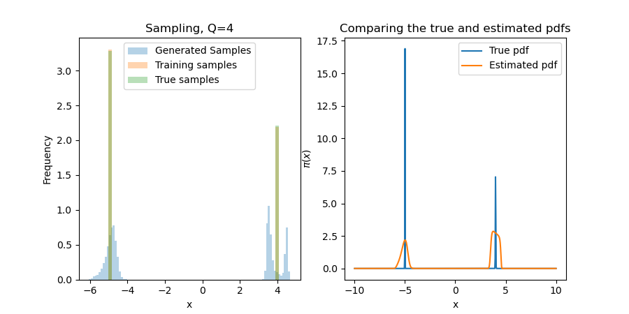
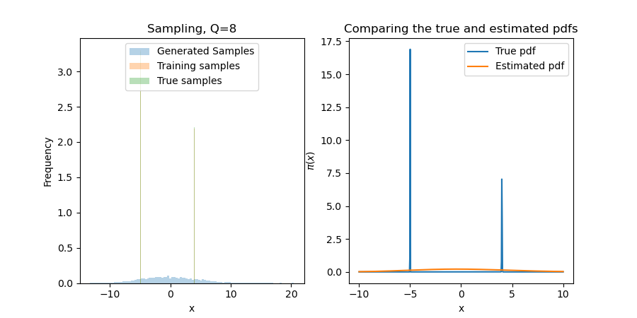
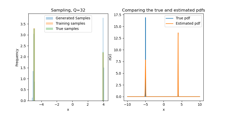
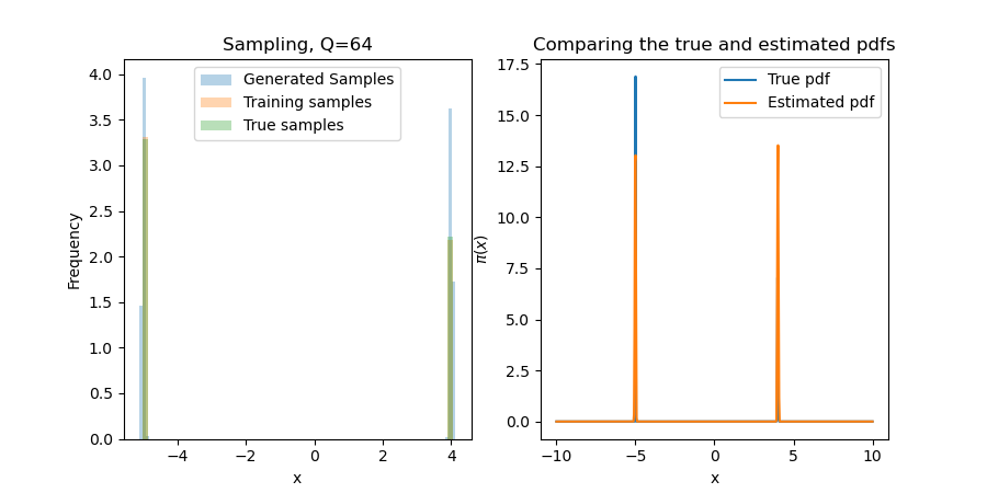
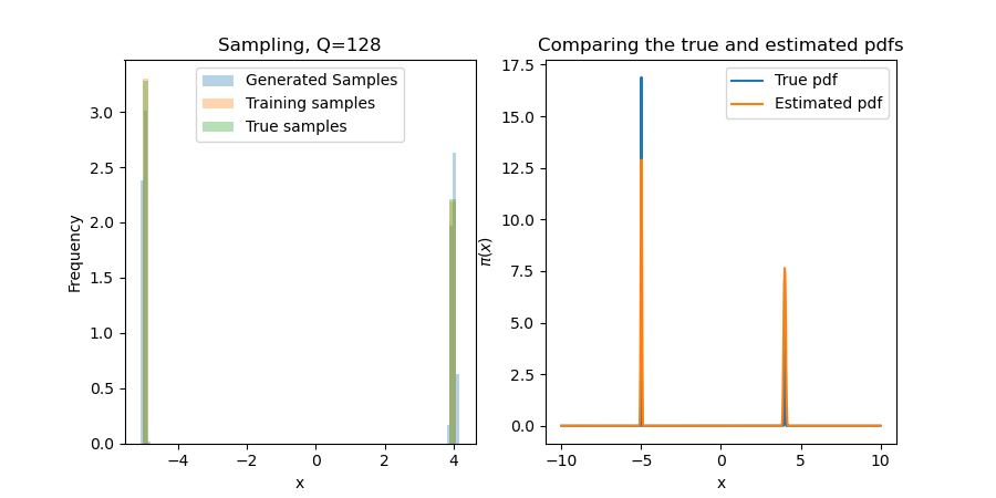
We sample by using a bisection search with 50 iterations. This narrows down the inversion area exponentially, so if we assume a support of $[-10,10]$, we will find a point that is within $20(2^{-50}) \approx 10^{-15}$ of the true inversion value for the found map (which is itself only an approximation of the true map). The major problem here is that this true distribution is difficult for any transport map to approximate (in particular, it is impossible to find a deterministic map $S$ for a discrete distribution), and so we often assign a value in the wrong bin when it is on the cusp of a near-discontinuity in $S$.

Two-dimensional example

This mostly demonstrates that my Pytorch code works in multiple dimensions; further, it illustrates conditional samples by amortization. We train a map $S(x_1,x_2) = (S_1(x_1),S_2(x_1,x_2))$ on joint samples $(X_1,X_2)\sim\pi$. If we now want to generate samples conditioning the first coordinate as some fixed $y^*$, we generate $Z^{(i)}\sim\mathcal{N}(0,1)$ and find $X^{(i)} = S_2 (y^*,\cdot)^{-1} (Z^{(i)})$ such that $X^{(i)} \sim \pi^{(2)} (x_2|x_1=y^*).$ Here we use $Q=16$.

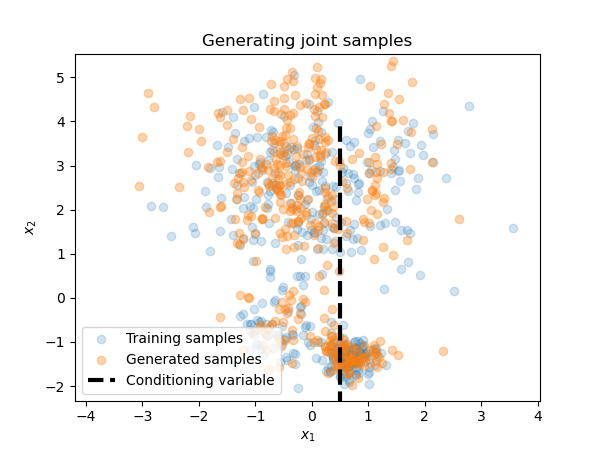
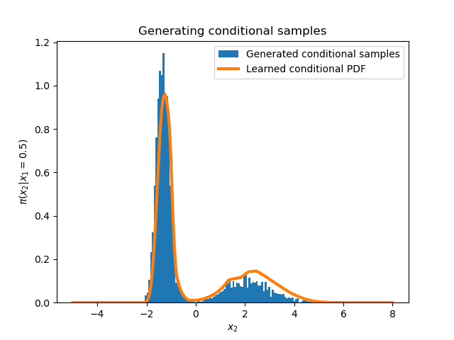
While the learned PDF does not look exactly like a Gaussian mixture (unlike the true conditional of $\pi$), it remains controlled in the tails and generates feasible samples with "only" $N=5000$.

Infinite dimensional example

It seems melodramatic to jump from two to infinite dimensions, but here we try to solve a common simulation-based inference problem constrained by partial differential equations (PDEs). Consider the following PDE \[\nabla\cdot(\exp(\kappa(x,\omega))\, \nabla u(x,\omega)) = s(x)\quad\forall x\in(0,1),\quad \partial_x u(0,\omega) = F,\quad u(1,\omega) = D.\]

We infer the log-diffusion field $\kappa(x,\omega)$, which we parameterize in a class of Gaussian random fields. Skipping many details one could find in, e.g., (Marzouk, Najm 09), we represent $\kappa$ by the truncated Karhunen-Loeve (KL) expansion of a Gaussian process \[\kappa(x,\omega) = \sum_{j=1}^d \psi_j(x)Z_j(\omega),\] where the (non-stochastic) functions $\psi_j$ determine a covariance function $C(x,y)$ such that $\mathbb{C}\mathrm{ov}(\kappa(x,\omega),\kappa(y,\omega)) = C(x,y)$ and $Z_j$ are independently and identically Gaussian-distributed. We choose $C(x,y) = \exp(-|x-y|/\ell)$ as our covariance function with $\ell=0.3$. This induces nondifferentiable realizations of $\kappa$. A few of these realizations and induced solutions are below.

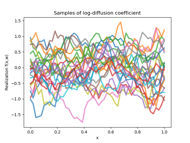
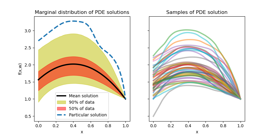
The solution highlighted on the left is induced by some particular realization of the diffusion field that we would like to infer. First, we take ten thousand simulations of the PDE induced by independent realizations of the KL expansion (simulated using the Nystrom method with 150 quadrature points). Since it is unrealistic to be able to access the analytical PDE solution everywhere, we instead take five evenly spaced points in the domain $(0,1)$ and assume normally-distributed noise with variance 0.025. Truncating at 40 KL coefficients, we learn a triangular map $S:\mathbb{R}^{5}\times\mathbb{R}^{40}\to\mathbb{R}^{40}$, i.e., we amortize the conditional inference over all possible observations by employing "pushforward-based inference". A triangular map here is natural; the KL coefficients come from a sort of Gram-Schmidt-like orthogonalization process, and thus most of the variance in truly smooth diffusion fields will be attributable to the first few KL coefficients.

After a training routine (100 epochs of SGD), we attempt to infer the diffusion field with the discontinuous derivative that generated the highlighted solution above with mixed results. The KL coefficients do not seem to concentrate around the correct area unfortunately, where we see joint-marginals of generated samples shown below for the first seven conditionally generated KL modes. Below that, we visualize a few generated diffusion fields and compare them to the diffusion field that generated the data in black; we also do so for the predictive distribution over the PDE solutions conditioned on the observation value.

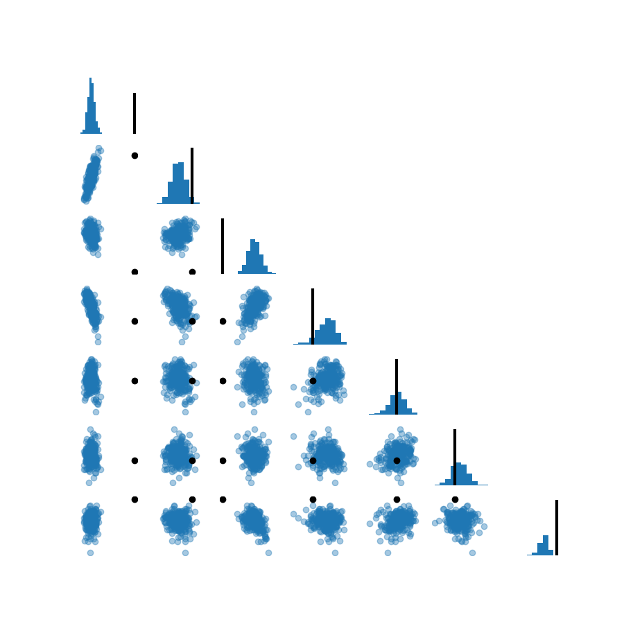
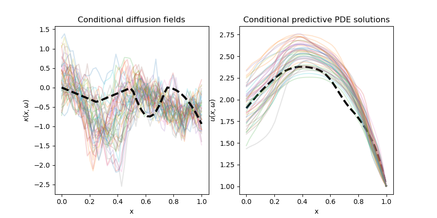
Unfortunately, it looks like the transport map hasn't yet converged. While the loss convergence is not illuminating in any standalone figure, it does seem like the optimization was not quite done after our 100 epochs with a learning rate of 0.001. Future work would certainly be to optimize the map over a much longer period and do a more careful hyperparameter search. The upside is that, even for a partially trained map, we still do not seem to need to be particularly careful about the tails of the distribution. We also scale to higher dimensions much better than polynomials; we only used a network with 12960 parameters, which is leagues below the dimensionally-exponential growth of the polynomial basis.

Conclusions

While this blog post may have overstayed its welcome, it is certainly clear that these MRNNs are a viable alternative to polynomials in both lower and higher dimensions, given enough samples. This post only touches on different possibilities with such maps, and it is exciting to consider comparing results with different state-of-the-art methods which I didn't have time to train for these particular problems. The MRNNs that I show here seem capable enough to perform conditional inference quickly; the questions of sample efficiency, convergence, and a good validation procedure were not as readily addressed as I would have hoped just due to the time and space constraints of this project. I do hope to address all of these things in the future, and I do believe that these are tractable for uses across many different areas.